A correlation analysis is a statistical procedure that evaluates the association between two sets of variables. The association between variables can be linear or nonlinear. In communication research, however, correlation analyses are mostly used to evaluate linear relationships. Sets of variables may include one or many variables. Associations between two variables (two sets of one variable) can be analyzed with a bivariate correlation analysis. Associations between one (dependent) variable and a set of two or more (independent) variables can be studied using multiple correlation (regression) analysis. Relationships between sets of many (independent and dependent) variables can be investigated using canonical correlation analysis.
Variables in each set can be measured on a nominal, ordinal, or interval level. There is a specific correlation analysis for any combination of measurement level and number of variables in each set. Associations between ordinal variables (i.e., variables that have been measured on an ordinal level) are usually analyzed with a nonparametric correlation analysis. All other combinations can be considered parametric linear correlation analyses and are as such special cases of canonical correlation analysis. Among the quantitative research methodologies, correlation analyses are recognized as one of the most important and influential data analysis procedures for communication research and for social science research in general. Explanation and prediction are generally considered the quintessence of any scientific inquiry. One can use variables to explain and predict other variables only if there is an association between them. One of the most established and widely applied correlation analyses is the bivariate linear correlation analysis, which will be used in the following demonstration.
Bivariate Linear Correlation Analysis – Product–Moment Correlation Coefficient
Suppose the researchers are interested in the relationship between the variables “playing a violent video game” (X) and “aggression” (Y). Both variables are measured on an interval level (X in hours per week; Y in aggression scores from 0 to 10) and with standard measurement instruments. The following dataset was obtained from five research participants:

Formula 1
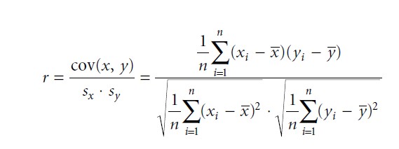
Since the researchers are interested in the linear relationship between the two interval variables they will apply a bivariate linear correlation analysis and calculate a bivariate correlation coefficient. A widely used bivariate correlation coefficient for linear relationships is the Pearson correlation coefficient, which is also known as product – moment correlation or simply as Pearson’s r:

Formula 2
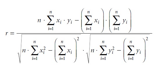
cov(x, y) means the covariance between the variable X and Y while sx and sy stand for the standard deviation of X and Y. The means of X and Y are indicated by ≈ and ¥. Hence, the product–moment correlation is simply a standardized covariance between two interval variables, or the covariance divided by the product of the variables’ standard deviation. For calculations it is recommended to use the following formula:
 Formula 3
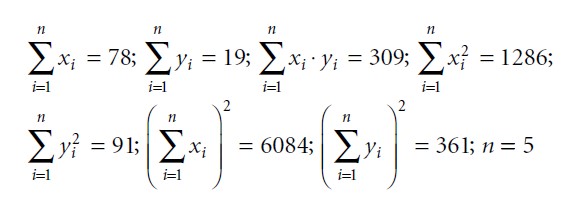
Therefore, we calculate the following sums and products:

Formula 4
Inserting these sums and products into the formula results in

Formula 5
This result indicates a positive product–moment correlation of 0.35 between “playing time of a violent video game” and aggression scores. All statistical software packages, such as SPSS, SAS, S-PLUS, R, and STATISTICA, offer a procedure for the calculation of product–moment correlations and many other correlation coefficients. The statistic software R is freely available at www.r-project.org.
Interpretation Of A Product–Moment Correlation Coefficient
The product–moment correlation coefficient (as most other correlation coefficients) will be a value between -1 and +1. A value of 0 indicates that the two variables are independent, i.e., have nothing in common. A value of both +1 and -1 would be interpreted as a perfect linear relationship between the two variables. A correlation of +1 stands for a positive or increasing linear relationship (“the more of variable X the more of variable Y” or vice versa). A correlation of −1 represents a negative or decreasing linear relationship (“the more of variable X the less of variable Y” or vice versa). The closer the correlation coefficient is to either −1 or + 1 the stronger the association between the two variables.
The squared correlation coefficient indicates the proportion of common variance between the two variables and is called the coefficient of determination. In the example above, the squared product–moment correlation is 0.352 = 0.1225, or 12.25 percent. This means that the two variables “playing time of a violent video game” (X) and “aggression” (Y) share 12.25 percent of their variance. In other words, 12.25 percent of variable Y is redundant when knowing variable X or vice versa. This result, however, also means that 100 percent minus 12.25 percent = 87.75 percent of the variables’ variance is not shared and needs to be explained by other variables. This quantity is commonly called the coefficient of alienation.
Many authors have suggested guidelines for the practical interpretation of a correlation coefficient’s size. The question is whether a given correlation coefficient indicates a small, medium, or strong association between variables. Cohen (1988), for example, has suggested the following categorization of correlation coefficients for psychological research: 0.10 < r < 0.29 or −0.29 < r < −0.10 indicates a small correlation (small effect), 0.30 < r < 0.49 or −0.49 < r < −0.30 a medium correlation (medium effect), and 0.50 < r < 1.00 or −1.00 < r < −0.50 a strong correlation (strong effect). As Cohen stated himself, these guidelines are, to a certain degree, arbitrary and should not be taken too seriously. Ultimately, the interpretation of a correlation coefficient’s size depends on the context. On the one hand, a correlation coefficient of 0.85 may indicate a weak relationship if one is studying a physical law with highly reliable measurement instruments. On the other hand, a correlation coefficient of 0.35 may indicate a strong relationship if many other variables intervene in the association of two or more variables, or if one has to use measurement instruments with imperfect reliability. A categorization of correlation coefficients that is comparable to Cohen’s classification and based on communication research findings is still missing.
Significance Of A Product–Moment Correlation Coefficient
The above example of a product–moment correlation resulted in a product–moment correlation coefficient of 0.35 in a sample of five research participants. Most of the time, however, researchers are more interested in whether a result found in a sample can be generalized to a population. In other words: researchers are often interested in whether hypotheses that refer to relationships among variables in a population hold when confronted with empirical data in a sample. For this purpose, one has to apply a statistical significance test. The classical hypotheses of a product–moment correlation coefficient are:
Two-sided research hypothesis (H1; association existent): ρ ≠ 0
Two-sided null hypothesis (H0; no association existent): ρ = 0
One-sided research hypothesis (H1; positive/negative association): ρ > 0 or ρ < 0
One-sided null hypothesis (H0; no or negative/no or positive association): ρ ≤ 0 or ρ ≥ 0
In the example above we assume a one-sided research hypothesis, i.e., we assume a positive correlation between the variables “playing time of a violent video game” and “aggression.” In other words, we expect that the more often people play a violent video game the higher their aggression levels, or vice versa. A null hypothesis test for r can be performed using a t or F sampling distribution. We obtain the t or F statistic as:

Formula 6
As one can see, t =√F . If the null hypothesis is true, the F statistic is Fisher’s F distributed with df1 = 1 and df2 = n − 2 degrees of freedom, or the t statistic is student’s t distributed with df = n − 2 degrees of freedom. According to the corresponding sampling distributions, the probability of finding a t value of 0.645 or an F value of 0.416 under the assumption of a true null hypothesis is p = 0.282. Since p values of greater than α = 0.05 (5 percent) usually do not result in the rejection of the null hypothesis, the relationship in the sample is characterized as not significant.
The Pitfalls Of Correlation Analysis
The concept of correlation analysis and correlation coefficients in particular can be easily misconceived. The following three aspects are frequently a source of misinterpretations:
Correlation Analysis and Linearity: Most correlation analyses indicate only linear relationships among variables and will miss nonlinear associations. For example, a perfectly U-shaped relationship between two interval variables will result in a product– moment correlation coefficient of zero and, therefore, would suggest no association. Hence, it is important to test whether the relationship under examination could be nonlinear in nature before conducting a linear correlation analysis. Among various statistical procedures, one can use a simple scatterplot for this purpose.
Correlation Analysis and Systematic Sample Biases: A correlation analysis with a test of statistical significance assumes that we have a perfect random sample at hand. Frequently, however, this is not the case. For example, samples can be composed of extreme groups, or samples may not cover the entire variation of variables in a population. While extreme group selection usually leads to an overestimation of the true relationship in a population, samples that are restricted in variation typically result in an underestimation of a correlation in a population. Another problem is that correlation coefficients are extremely sensitive to outliers in a sample which, too, lead to an overestimation of a population’s true correlation. It is recommended to check a sample for systematic sample biases before conducting a correlation analysis.
Correlation Analysis and Causality: The most common misconception of a correlation analysis, however, refers to the question of causality. The fact that two or more variables are correlated does not mean that some variables can be considered as cause and others as effect. Correlation is not causation! The example above stated a positive correlation between “playing time of a violent video game” and “aggression.” It is possible that playing a violent video game causes higher aggression scores (effect hypothesis), but it is also conceivable that already aggressive personalities purposely select violent video games (selection hypothesis). A positive product–moment correlation coefficient does not provide any information about which of the two competing hypotheses is the better model. Perhaps both variables are even affected by a third variable and show no direct relationship at all. In this case the association between “playing time of a violent video game” and “aggression” would be a spurious relationship. On a basic level, three conditions define causality:
1 Time order must be appropriate. If X is the cause and Y the effect, then usually X antecedes Y in time.
2 Variation must be concomitant, as shown with a significant correlation coefficient.
3 The relationship among variables must not be explained by other variables, i.e., is not spurious.
Considering these three conditions, a significant correlation coefficient is a necessary, but not a sufficient, condition for causality.
References:
- Abdi, H. (2007). Coefficients of correlation, alienation and determination. In N. J. Salkind (ed.), Encyclopedia of measurement and statistics. Thousand Oaks, CA: Sage.
- Agresti, A., & Finlay, B. (1997). Statistical methods for the social sciences, 3rd edn. Upper Saddle River, NJ: Prentice Hall.
- Chen, P. Y., & Popovich, P. M. (2002). Correlation: Parametric and nonparametric measures. Sage university papers series on quantitative applications in the social sciences no. 139. Thousand Oaks, CA: Sage.
- Cohen, J. (1988). Statistical power analysis for the behavioral sciences. Hillsdale, NJ: Lawrence Erlbaum.
- Cohen, J., Cohen, P., West, S. G., & Aiken, L. S. (2002). Applied multiple regression/correlation analysis for the behavioral sciences, 3rd edn. Mahwah, NJ: Lawrence Erlbaum.
- Miles, J., & Shevlin, M. (2004). Applying regression and correlation: A guide for students and researchers. Thousand Oaks, CA: Sage.
- Thompson, B. (1984). Canonical correlation analysis: Uses and interpretation. Sage university papers series on quantitative applications in the social sciences no. 47. Thousand Oaks, CA: Sage.
